Halloween Pictures - Period 1

Here are the pictures of our wonderful door decorating and pumpkin carving... Period 1 :)






































HAVE A GOOD HALLOWEEN EVERYONE!

3.4 Solving Rational Equations, Solving Rational Inequalities – Period 1

Today’s lesson was about solving rational inequalities and equations

How to solve rational Equations:

Technically what are you doing? You are trying to find the value of x that allows both equations to be equal.
Example:
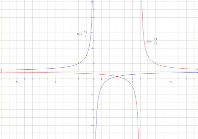
Graphically:
1) Graph both equations.
2) Find the point(s) of intersection (POI)
3) State the restrictions
The red line represents f(x) = (x-4) / (x-6)
The blue line represents g(x) = (x-2) / x
As you can visually inspect, the point of intersection is at x = 3.

⁂ x = 3, when x ≠ 0, 6

Algebraically:
1) Factor numerator and denominator if necessary
2) Cross multiply
3) Simplify to obtain polynomial equations
4) Solve for x
5) State the restrictions

How to solve rational inequalities:

Technically what are you doing? You are trying to find the values of x that satisfy the equation.

Example:
1) Bring all values to one side, resulting on one side equaling to 0

2) Simplify and factor the numerator and denominator
3) Find the vertical asymptotes, zeros, and restrictions

Vertical asymptotes: x = -5, -6
Zeros: 4, -1

4) Create a number line
5) Plot the vertical asymptote, zeroes (These are the factors the can affect the sign of the function)
6) Use test points to determine the sign of the expression in each interval.
7) State the solution


*NOTE: an equality symbol acts like an equal sign. However, DO NOT crosses multiply, when solving rational inequalities. When multiplying an inequality by a negative value, the greater or less than sign must be switched around.

Algebraically Summary:

1) Bring all values to one side, resulting on one side equaling to 0
2) Simplify and factor the numerator and denominator
3) Find the vertical asymptotes, zeros, and restrictions
4) Create a number line
5) Plot the vertical asymptote, zeroes (The function may change at the zeros or at vertical asymptotes. )
6) Use test points to determine the sign of the expression in each interval.
7) State the solution, with the restriction.

This is the file for the above note

3.3 Rational Functions of the form f(x)=(ax+b) / (cx+d)

Today we had a supply and therefore there was no lesson, just a handout. Since we didn't have any verbal explanations of today's lesson, I will just re-write the key points of the handout.

Previously, we had only touched upon reciprocal functions. Basically, that's the inverse of a function that we are used to - for example, x^2-3x+2 is a function that we are used to, and the inverse of this function (or the reciprocal) would be 1/(x^2-3x+2). In a reciprocal function, 1 is divided by a polynomial.

The handout that we received today discussed functions that are also rational, except both the numerator and the denominator of the function are "polynomials in x of degree n and m" (from the sheet).
The general formula for a function of this sort is:
f(x) = (ax^n + b) / (cx^m + d).


We still need to be able to discuss the key points of functions of this nature, including the x- and y- intercepts, as well as both the horizontal and vertical asymptotes. We also need to be able to describe the way the function acts as it approaches the asymptotes from all sides.

• To determine the x-intercept of any rational function, we just set y=0 and solve for x. Similarly, to determine the y-intercept, we set x=0 and solve for y.
• To determine the vertical asymptote of rational functions, we set the denominator equal to 0 and solve for the possible value(s) of x.

Neither of these have changed from reciprocal functions to functions of the form f(x)=(ax+b) / (cx+d) (which we are looking at now). The only difference between the two lies in the way we determine the horizontal asymptote.
There are two methods in determining this. The most simple one comes in the form of general rules: (Remember, n and m are the exponents on the x values in the equation)

1. If n < m, y="0
2. If n = m, the horizontal asymptote is y = (coefficient of the x^n term) / (coefficient of the x^m term) <-- one thing that I got messed up on in the homework is to make sure you look at the COEFFICIENT (the term paired with the x) and not the constant.
3. If n > m, there is no horizontal asymptote.

The second is to create a table of values, using large positive numbers ("close" to positive infinity) and large negative numbers ("close" to negative infinity) and determine the y values, and seeing how close they get to a number without touching (property of an asymptote).

Once you have your asymptotes and intercepts, you can sketch your graph. In terms of which way to draw the graph (end behaviours), I just create a table of values (like the second method for determining the horizontal asymptote) and plot the points that way. There might be an easier way but I guess I haven't found it yet so that works for now.

3.2 Reciprocal of a Quadratic Function- Period 3/4

Friday’s lesson was analyzing the reciprocal function of a quadratic function. With a linear function we took, for instance, y= x-7 and flipped it to be y= 1/ (x-7). The same goes for y= 2x+27 which in turn would be 1/(2x+27).

Because we are continuing with the theme of reciprocals, the same trend occurs with quadratic function, y= x ^2. The reciprocal of this function, just as it was with linear functions, is y= 1/ (x^2). Not too difficult, eh?

Now that we have our equation established, anything is possible. However rather than establishing rules to memorize, we’ll refer the now infamous comparison chart, which we have already done successfully in class for both linear and quadratic functions, to discuss the reasons for such similarities and differences. Why do the same concepts apply to both linear and quadratic functions and their reciprocals?

We’ll use the example y= 1/ x^2-4, shown above. I sincerely apologize for both graphs being in red.

• Let’s first start with the zeros, or x-intercepts, of our function 1/x^2-4, which are -2 and 2. In these cases, the y-value of this coordinate is 0. When we apply this to the reciprocal, the denominator becomes 0, making the fraction 1/0, which doesn’t really work. So, two vertical asymptotes are created, in which the graph comes near however does not touch the x-values of 2 and -2.Next is the y-intercept, in which the x value is always 0 and for the quadratic function, the y-intercept is -4 while the reciprocal is, of course, -1/4.

• Next are positive and negative intervals, which seem to follow the same trend for both linear and quadratic reciprocals. Why? Because if an x-value is positive, the reciprocal will of course be positive because the sign of the value is not changing. 2 will be 1/2 and -2 will be -1/2.

• Lastly we’ll briefly review increasing and decreasing intervals. Simply put, as the x-values for the quadratic function increase, the reciprocals for these values decrease.

1----->1

2-----> 1/2

3-----> 1/3

As the graph of the quadratic moves UP the reciprocal function moves DOWN. As the quadratic function INCREASES our reciprocal DECREASES.

1/2-----> 2

1/3-----> 3

As you can see, the same goes for fractions and negative x-values of our quadratic function and the x-values of the reciprocal quadratic function. As the x-values of the quadratic function DECREASE, the values of the reciprocal function INCREASE.

****For Ms. Burchat’s period 3/4 class:****

If you still don’t see the importance of conceptual understanding, recall her university horror story and be scared into caring about conceptual understanding! And another lifelong rule? Don’t let anyone call you slave.... Or esclave, servus, or esclavo. Or even sklave or abed for that matter.

And for some comic relief, check this out...

Don’t ask me how I found it. =)

http://www.youtube.com/watch?v=Ooa8nHKPZ5k

Characteristics of Quadratic Reciprocal Functions

Review
In the last two lessons we have talked about reciprocal functions. To review a reciprocal is the flip of any regular function of a function in the form 1/f(x) instead of just f(x). Some easy examples of reciprocals are things like the reciprocal of 2 is 1/2, and 3 is 1/3. A reciprocal function is y=x+2, and y=1/(x+2).

Quadratic reciprocals
A quadratic reciprocal is the same as an ordinary reciprocal function ex. y=x^2 +2, y=1/(x^2+2). It also follows the same rules as a regular degree 1 reciprocal function:

• The zeros (or x-intercepts) of a quadratic will be the asymptotes of the reciprocal function. Just like in a degree 1 reciprocal function except for the fact that for some quadratics there are 2 zeros, instead of just 1. Reason: You cannot have 1/0 it does not work. So on the original graph, f(x), the only values that made the equation =0 were the x-intercepts. This means the x intercepts cannot happen on a reciprocal graph or else it would equal 1/0.
  
• When the regular quadratic has positive y values the reciprocal function will also have positive y values, same for negative. Reason: 2 is +, 1/2 (its reciprocal) is also positive. -2 is -, -1/2 its reciprocal is also negative.
  
• Where the original graph is increasing (from left to right) the reciprocal function will be decreasing and the opposite. Reason: 2 the reciprocal is 1/2, 3 the reciprocal is 1/3, 4 is 1/4, and 5 is 1/5. This shows that as the original gets bigger the reciprocal gets smaller showing why as one graph increases the other decreases.
  
• Finally all the points on the original graph have reciprocal points on the second graph.
  

These 4 common rules for all reciprocal functions once mastered will allow you to always graph a reciprocal function. I was going to make 2 graphs to show but I have no idea how??? Some one tell me on Monday and I can make it better but until then this is all I've got.

Characteristcs of rational functions

Rational functions are in the form f(x)= P(x)/Q(x) where P(x) and Q(x) are polynomial functions and Q(x) is degree 1 or higher. The simplest rational function is f(x)= 1/x.

As you can see the graph does not cross the x or y axis and so we have vertical and horizontal asymptotes. An ASYMPTOTE is a line that the graph approaches more and more closely but never touches.

When we compare graphs of the base function y=x to y=1/x there are many patterns. Whatever the x intercept of the linear function is will equal the vertical asymptote of the rational function. The section where there are positive intervals are always the same for the linear and rational function. Also if there are all increasing intervals (so the linear function is going up) than the reciprocal function will have the opposite, all decreasing. However, x will never be able to equal where the asymptote is. For example in f(x)= 1/x x cannot equal 0.

Solving Inequalities, October 18, 2009, Tobias Budirahaju, Period 1

In the past few days we have been learning how to solve inequalities in class. We have learned two main methods on how to solve inequalities. One using technology, and one algebraically.

Technology:
when using technology to solve inequalities you would usually use a graphing calculator. You would plug the equation into the graphing calculator and then graph it. Using the resulting graph you would be able to determine the answer to solve inequalities because the graph will give you important information such as x intercepts, the co-ordinates of specific points and etc.

Algebraically:
When solving inequalities algebraically there is two different methods you can choose from. The first method is that you can graph the function. Graphing the function will allow you to solve for inequalities the same way technology would, by graphing you will see the graph and all the points, thus giving you the necessary information needed to solve the question being asked. However you can also solve the inequality by using strictly algebra. First you would take the equation given and put it into factored form. Then you would figure out the characteristics of the graph by plugging in different x's that will tell you if the graph is positive or negative at that point.

Period 4: Solving Inequalities Algebraically

Inequality deals with a range of values, rather than an exact number, so it is necessary to replace the equal sign in an equation with its supposed inequality (either >, <, >, or <).

For example, Solve for the following inequality:

(x + 10) (2x – 9) > 0

1. Break up both of the brackets into two separate “sections”, x +12>0 and 2x - 9 >0.
2. So far, we know that each individual section must exceed the value of 0, as this is the inequality. From this, we can isolate the x value to determine the roots.
   
   x+ 12 > 0
   x > -10
   
   2x-9 >0
   = 2x> 9
   x > 9/2
   
   Note that for section 2, the value of x can also be 0.
   
   So now we know that the roots of the equation when (x + 10) (2x – 9) = 0 are x = -10, x = 9/2, and x = 0
   
   

3. We can then break up number line into three intervals in relation to the roots that we have found.
   
   Because the lowest root is -10, we recognize in order for the graph to continue negatively, x must therefore be less than -10, so x < -10.
   
   Likewise, the highest root value is 9/2 so in order for the graph to continue positively, x must be bigger than 9/2, so 9/2 > x. We must also notice that the middle interval must (graphically) be larger than -10, yet smaller than 9/2, so, respectively, the inequality is represented by -10 <>
   
   
   
4. You can test out each interval by plugging it into the equation and determining which one is the solution.
   
   For x<-10, test x = -11
   (-11 + 10) (2 (-11) -9) = 31
   because the value “31” is greater than “0”, x< -10 is a solution. For -10 <9/2,>x = 1
   (1+10) (2(1)-9) = -77
   because the value “-77” is less than “0”, -10 <> solution. For x > 9/2, test x = 5
   (5+10) (2(5)-9) = 135
   because the value “135” is greater than “0”, x>9/2 is a solution.
   
   
5. Summarize the information found onto a table:
   

   Interval Factor	x < -10	-10	x > 9/2
   (x +10)	( - )	( + )	( + )
   (2x – 9)	( - )	( - )	( + )
   f(x)	( + )	( - )	( + )

   
   
6. The solution, shown on the number line, is x < -10 and x > 9/2

   

   Note: Page 8 of our textbooks summarizes all possible intervals
   
   

   Therefore, the solution is XE(-∞, -10] U[9/2, ∞)